Beating the binary search algorithm – interpolation search, galloping search
Binary search is one of the simplest yet most efficient algorithms out there for looking up data in sorted arrays. The question is, can it be beaten by more sophisticated methods? Let’s have a look at the alternatives.
In some cases hashing the whole dataset is not feasible or the search needs to find the location as well as the data itself. In these cases the O(1) runtime cannot be achieved with hash tables, but O(log(n)) worst case runtime is generally available on sorted arrays with different divide and conquer approaches.
Before jumping to conclusions, it is worth to note that there are a lot of ways to “beat” an algorithm: required space, required runtime, and required accesses to the underlying data structure can be different priorities. For the following runtime and comparison tests different random arrays between 10,000 and 81,920,000 items were created with 4 byte integer elements. The keys were evenly distributed with an average increment of 5 between them.
Binary search
 The binary search is a guaranteed runtime algorithm, whereas the search space is always halved at each step. Searching for a specific item in an array guaranteed to finish in O(log(n)) time, and if the middle point was selected luckily even sooner. It means that an array with 81,920,000 elements only needs 27 or less iterations to find the element’s location in the array.
Because of the random jumps of the binary search, this algorithm is not cache friendly so some fine tuned versions would switch back to linear search as long as the size of the search space is less than a specified value (64 or less typically). However, this final size is very much architecture dependent, so most frameworks don’t have this optimization.
Galloping search; galloping search with binary search fallback
 If the length of the array is unknown for some reason, the galloping search can identify the initial range of the search scope. This algorithm starts at the first element and keeps doubling the upper limit of the search range until the value there is larger than the searched key. After this, depending on the implementation, the search either falls back to a standard binary search on the selected range, or restarts another galloping search. The former one guarantees an O(log(n)) runtime, the latter one is closer to O(n) runtime.
Galloping search is efficient if we expect to find the element closer to the beginning of the array.
Sampling search
 The sampling search is somewhat similar to the binary search but takes several samples across the array before deciding which region to focus on. As a final step, if the range is small enough, it falls back to a standard binary search to identify the exact location of the element.
The theory is quite interesting but in practice the algorithm doesn’t perform too well.
Interpolation search; interpolation search with sequential fallback
 The interpolation search supposed to be the “smartest” among the tested algorithms. It resembles the way humans are using phonebooks, as it tries to guess the location of the element by assuming that the elements are evenly distributed in the array.
As a first step it samples the beginning and the end of the search space and then guesses the element’s location. It keeps repeating this step until the element is found. If the guesses are accurate, the number of comparisons can be around O(log(log(n)), runtime around O(log(n)), but unlucky guesses easily push it up to O(n).
The smarter version switches back to linear search as soon as the guessed location of the element is presumably close to the final location. As every iteration is computationally expensive compared to binary search, falling back to linear search as the last step can easily outperform the complex calculations needed to guess the elements location on a short (around 10 elements) region.
One of the big confusions around interpolation search is that the O(log(log(n)) number of comparisons may yield O(log(log(n)) runtime. This is not the case, as there is a big tradeoff between storage access time versus CPU time needed to calculate the next guess. If the data is huge and storage access time is significant, like on an actual disk, interpolation search will easily beat binary search. However, as the tests show, if access time is very short, as in RAM, it may not yield any benefit at all.
Test results
All the code was hand written for the tests in Java (source code at the end); each test was run 10 times on the same array; the arrays were random, in memory integer arrays.
The interpolation search fell back to linear search if the assumed distance was 10 or fewer items, while the sampling search took 20 samples across the search space before deciding where to continue the search. Also, when the key space was less than 2000 items, it fell back to standard binary search.
As a reference, Java’s default Arrays.binarySearch was added to compare its runtime to the custom implementations.
Despite of the high expectations for interpolation search, the actual runtime did not really beat the default binary search. When storage access time is long, a combination of some kind of hashing and B+ tree probably would be a better choice, but it is worth to note that on uniformly distributed arrays the interpolation search combined with sequential search always beats the binary search on the number of comparisons required. It’s also interesting how efficient the platform’s binary search was, so for most cases it’s probably not worth it to replace it with something more sophisticated.
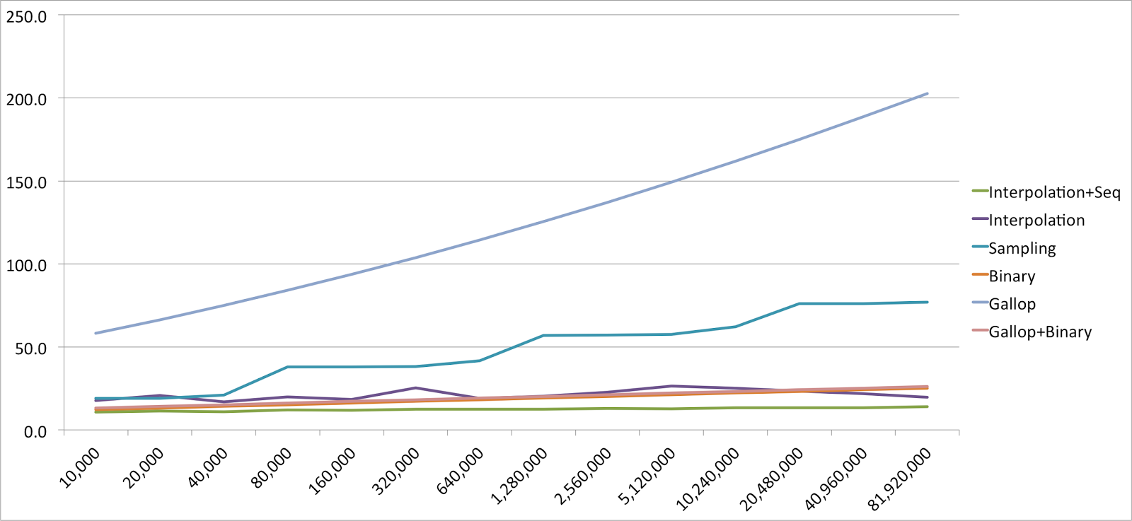
Raw data – average runtime per search
Raw data – average number of comparisons per search
In some cases hashing the whole dataset is not feasible or the search needs to find the location as well as the data itself. In these cases the O(1) runtime cannot be achieved with hash tables, but O(log(n)) worst case runtime is generally available on sorted arrays with different divide and conquer approaches.
Before jumping to conclusions, it is worth to note that there are a lot of ways to “beat” an algorithm: required space, required runtime, and required accesses to the underlying data structure can be different priorities. For the following runtime and comparison tests different random arrays between 10,000 and 81,920,000 items were created with 4 byte integer elements. The keys were evenly distributed with an average increment of 5 between them.
Binary search
Because of the random jumps of the binary search, this algorithm is not cache friendly so some fine tuned versions would switch back to linear search as long as the size of the search space is less than a specified value (64 or less typically). However, this final size is very much architecture dependent, so most frameworks don’t have this optimization.
Galloping search; galloping search with binary search fallback
Galloping search is efficient if we expect to find the element closer to the beginning of the array.
Sampling search
The theory is quite interesting but in practice the algorithm doesn’t perform too well.
Interpolation search; interpolation search with sequential fallback
As a first step it samples the beginning and the end of the search space and then guesses the element’s location. It keeps repeating this step until the element is found. If the guesses are accurate, the number of comparisons can be around O(log(log(n)), runtime around O(log(n)), but unlucky guesses easily push it up to O(n).
The smarter version switches back to linear search as soon as the guessed location of the element is presumably close to the final location. As every iteration is computationally expensive compared to binary search, falling back to linear search as the last step can easily outperform the complex calculations needed to guess the elements location on a short (around 10 elements) region.
One of the big confusions around interpolation search is that the O(log(log(n)) number of comparisons may yield O(log(log(n)) runtime. This is not the case, as there is a big tradeoff between storage access time versus CPU time needed to calculate the next guess. If the data is huge and storage access time is significant, like on an actual disk, interpolation search will easily beat binary search. However, as the tests show, if access time is very short, as in RAM, it may not yield any benefit at all.
Test results
All the code was hand written for the tests in Java (source code at the end); each test was run 10 times on the same array; the arrays were random, in memory integer arrays.
The interpolation search fell back to linear search if the assumed distance was 10 or fewer items, while the sampling search took 20 samples across the search space before deciding where to continue the search. Also, when the key space was less than 2000 items, it fell back to standard binary search.
As a reference, Java’s default Arrays.binarySearch was added to compare its runtime to the custom implementations.
 |
| Average search time / element, given the array size |
 |
| Average comparisons / search, given the array size |
Despite of the high expectations for interpolation search, the actual runtime did not really beat the default binary search. When storage access time is long, a combination of some kind of hashing and B+ tree probably would be a better choice, but it is worth to note that on uniformly distributed arrays the interpolation search combined with sequential search always beats the binary search on the number of comparisons required. It’s also interesting how efficient the platform’s binary search was, so for most cases it’s probably not worth it to replace it with something more sophisticated.
Raw data – average runtime per search
| Size | Arrays. binarySearch | Interpolation +Seq | Interpolation | Sampling | Binary | Gallop | Gallop +Binary |
|---|---|---|---|---|---|---|---|
| 10,000 | 1.50E-04 ms | 1.60E-04 ms | 2.50E-04 ms | 3.20E-04 ms | 5.00E-05 ms | 1.50E-04 ms | 1.00E-04 ms |
| 20,000 | 5.00E-05 ms | 5.50E-05 ms | 1.05E-04 ms | 2.35E-04 ms | 7.00E-05 ms | 1.15E-04 ms | 6.50E-05 ms |
| 40,000 | 4.75E-05 ms | 5.00E-05 ms | 9.00E-05 ms | 1.30E-04 ms | 5.25E-05 ms | 1.33E-04 ms | 8.75E-05 ms |
| 80,000 | 4.88E-05 ms | 5.88E-05 ms | 9.88E-05 ms | 1.95E-04 ms | 6.38E-05 ms | 1.53E-04 ms | 9.00E-05 ms |
| 160,000 | 5.25E-05 ms | 5.94E-05 ms | 1.01E-04 ms | 2.53E-04 ms | 6.56E-05 ms | 1.81E-04 ms | 9.38E-05 ms |
| 320,000 | 5.16E-05 ms | 6.13E-05 ms | 1.22E-04 ms | 2.19E-04 ms | 6.31E-05 ms | 2.45E-04 ms | 1.04E-04 ms |
| 640,000 | 5.30E-05 ms | 6.06E-05 ms | 9.61E-05 ms | 2.12E-04 ms | 7.27E-05 ms | 2.31E-04 ms | 1.16E-04 ms |
| 1,280,000 | 5.39E-05 ms | 6.06E-05 ms | 9.72E-05 ms | 2.59E-04 ms | 7.52E-05 ms | 2.72E-04 ms | 1.18E-04 ms |
| 2,560,000 | 5.53E-05 ms | 6.40E-05 ms | 1.11E-04 ms | 2.57E-04 ms | 7.37E-05 ms | 2.75E-04 ms | 1.05E-04 ms |
| 5,120,000 | 5.53E-05 ms | 6.30E-05 ms | 1.26E-04 ms | 2.69E-04 ms | 7.66E-05 ms | 3.32E-04 ms | 1.18E-04 ms |
| 10,240,000 | 5.66E-05 ms | 6.59E-05 ms | 1.22E-04 ms | 2.92E-04 ms | 8.07E-05 ms | 4.27E-04 ms | 1.42E-04 ms |
| 20,480,000 | 5.95E-05 ms | 6.54E-05 ms | 1.18E-04 ms | 3.50E-04 ms | 8.31E-05 ms | 4.88E-04 ms | 1.49E-04 ms |
| 40,960,000 | 5.87E-05 ms | 6.58E-05 ms | 1.15E-04 ms | 3.76E-04 ms | 8.59E-05 ms | 5.72E-04 ms | 1.75E-04 ms |
| 81,920,000 | 6.75E-05 ms | 6.83E-05 ms | 1.04E-04 ms | 3.86E-04 ms | 8.66E-05 ms | 6.89E-04 ms | 2.15E-04 ms |
Raw data – average number of comparisons per search
| Size | Arrays. binarySearch | Interpolation +Seq | Interpolation | Sampling | Binary | Gallop | Gallop +Binary |
|---|---|---|---|---|---|---|---|
| 10,000 | ? | 10.6 | 17.6 | 19.0 | 12.2 | 58.2 | 13.2 |
| 20,000 | ? | 11.3 | 20.7 | 19.0 | 13.2 | 66.3 | 14.2 |
| 40,000 | ? | 11.0 | 16.9 | 20.9 | 14.2 | 74.9 | 15.2 |
| 80,000 | ? | 12.1 | 19.9 | 38.0 | 15.2 | 84.0 | 16.2 |
| 160,000 | ? | 11.7 | 18.3 | 38.0 | 16.2 | 93.6 | 17.2 |
| 320,000 | ? | 12.4 | 25.3 | 38.2 | 17.2 | 103.8 | 18.2 |
| 640,000 | ? | 12.4 | 19.0 | 41.6 | 18.2 | 114.4 | 19.2 |
| 1,280,000 | ? | 12.5 | 20.2 | 57.0 | 19.2 | 125.5 | 20.2 |
| 2,560,000 | ? | 12.8 | 22.7 | 57.0 | 20.2 | 137.1 | 21.2 |
| 5,120,000 | ? | 12.7 | 26.5 | 57.5 | 21.2 | 149.2 | 22.2 |
| 10,240,000 | ? | 13.2 | 25.2 | 62.1 | 22.2 | 161.8 | 23.2 |
| 20,480,000 | ? | 13.4 | 23.4 | 76.0 | 23.2 | 175.0 | 24.2 |
| 40,960,000 | ? | 13.4 | 21.9 | 76.1 | 24.2 | 188.6 | 25.2 |
| 81,920,000 | ? | 14.0 | 19.7 | 77.0 | 25.2 | 202.7 | 26.2 |
Source code
The full Java source code for the search algorithms can be found here. Keep in mind, the code is not production quality; for instance, it may have too many or too few range checks in some cases!


You state: "One of the big confusions around interpolation search is that the O(log(log(n)) number of comparisons may yield O(log(log(n)) runtime" and "If the guesses are accurate, the number of comparisons can be around O(log(log(n)), runtime around O(log(n))"
ReplyDeleteThis is not correct.
Mind you that both 2*log(log(n)) and 1000000*log(log(n)) are both O(log(log(n)). For any constant c, c*f(n) is O(f(n)).
The c tends to be comparatively large in case of interpolation search vs other usual search algorithms. And it depends on implementation[*]. But with large enough n asymptotically faster algorithm will win.
If one looks at the performance data presented one could see that, when compared with example binary search code, example interpolation search has a lead of ~15% for n > 500000. Even built-in binary search (reliably faster that anything else) is virtually equal at the biggest n (n=81920000).
So yes, interpolation search will be faster when data is big enough. How big depends on how optimized implementation is[*], here it looks that it would be for n somewhere between 0.5 million and 100+ million.
There is other issue with interpolation search, not mentioned here:
while it's expected cost is O(log(log(n))), it's pessimistic cost is O(n). Try filling test arrays with numbers obtained the following way (of course sort it):
(int)Math.pow(62*Math.random(), 1.41)
*] Example implementation is not optimized. It converts back and forth between int and float (which is slow), it has extraneous ifs, etc...